 |
Upper Mississippi River Restoration ProgramLong Term Resource Monitoring |
|
 |
||
LTRM Statistics
Estimating Power to Detect Temporal Trends in LTRM Metrics
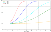
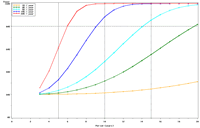
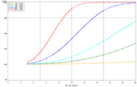
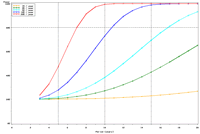
The selection of metrics for ecological programs naturally flows from the Program's goals and objectives. Once identified through the goals and objectives process, a set of potential metrics may be further refined through consideration of logistical and statistical considerations. One statistical consideration is the power to detect effects of management-important magnitudes. Statistical power represents the probability of detecting an effect—given a number of design and statistical details, and under the assumption that the effect is truly present. We accept that we may not always detect what is happening in the real world—but we would like the probability of detecting important effects to be as high as possible. Detecting an effect becomes more likely as (1) the magnitude of the effect increases, (2) variance decreases, (3) the number of samples increases, and (4) our acceptance of "false positives" increases. ("False positives" represent occasions when we decide something has changed but, in fact, the apparent change represents merely background variation.) We caution that power is a planning tool and is not generally considered useful retrospectively (i.e., once data have been collected; Hoenig and Heisey 2001). For this reason, this page addresses power to detect future effects only. Interest in past performance of the designs associated with LTRM metrics may be addressed by examining confidence intervals: mean or trend values contained within a given confidence interval appear reasonable while those outside the confidence interval do not (given the data and the selected Type I error rate). For example, a trend estimate with 90% confidence interval of 0.05 (0.01, 0.09) units suggests evidence against negative or negligible (<0.01 units) trend values but that trend values of, for example, 0.02 or 0.07 units are reasonable. This approach may best be coupled with an assignment of ecologically negligible effects. If, for the present example, ecologically negligible effects had been defined as less than 0.01 units in magnitude, we would see evidence for ecologically significant effects (because the confidence interval excludes effect values smaller than 0.01 units). A previous investigation examined the power to detect annual changes in a number of LTRM metrics. In the present investigation, we examine the power to detect long-term temporal trends in selected metrics. Given the typically relatively low cost of false positives for the LTRM, we assumed a false positive or Type I error rate of 20%. For discussion purposes, we have assumed adequate power to be defined as being greater than or equal to 80%. Power to detect trends of 1, 3, 5, 10, and 20% per year were estimated and for periods of 3 through 20 years. The following plots represent a sampling of the kind of power plots that can be created. For example, under the present sampling program, power to detect a 5% per year change in mayfly (Ephemeridae) relative abundance in Pool 13 reaches 80% after approximately 14 years (Figure 1b). This period decreases slightly to 13 years when sample size within sampling events is doubled and increases to 16 years when sample sizes are halved (Figures 1a, c). These small changes demonstrate an important issue: Given minimal sample sizes per year and variation in annual means that isn’t “explained” by a trend term, the sample size that really matters when estimating multi-year temporal trends is not the sample size per year but the number of years sampled. This is because temporal trends are estimated across annual means—and annual means, adjusted for trends, aren’t typically constant. Power to detect trends of a given magnitude was higher in Pools 4 and 13 than in Pool 26 (Figures 1b, 2). Reallocating the present macroinvertebrate sampling effort in Pool 13 entirely to a stratum with relatively low sampling variance (the impounded stratum) produces only minor effects on power to detect changes in mayfly relative abundance (Figure 1d). This is probably because the variance in the impounded stratum is similar to that in the backwater stratum and because the remaining strata (channel strata) represent only 10% of the Pool 13 sample area (for macroinvertebrates). Comments on power to detect trends for taxa groups other than mayflies are provided under the headings for those groups. |
|||
|
|
|||
| Figure 1. Estimated power to detect temporal trends in mayfly (Ephemeridae) relative abundance in Pool 13 under (a) half the present sampling intensity (n = 60), (b) the present sampling intensity (n = 120), (c) twice the present sampling intensity (n = 240), and (d) all present samples (n = 120) allocated to the impounded stratum. | |||
|
|
|||
|
Figure 2. Estimated power to detect temporal trends in mayfly (Ephemeridae) relative abundance under the present sampling intensity in (a) Pools 4 and (b) 26. |
|||
|
Bluegill (Lepomis macrochirus) Catch-per-unit Effort |
|||
|
Power to detect a 5% per year trend in bluegill catch-per-unit effort (CPUE) in Pool 4 is estimated to reach 80% after approximately 17 years; doubling and halving the present sample size will change this period to roughly 16 and 18 years, respectively (Figure 3). This relatively small influence of changes in sample size is explained by the relatively high proportion of annual variance attributable to real changes in bluegill CPUE means in Pool 4 (82%) and the consequently small proportion of interannual variation attributable to error or sampling variance (18%). These power plots are adjusted for moderate temporal correlation (r = 0.47) among annual bluegill CPUE means. Power estimated under a naive assumption of temporal independence, of course, appears higher (compare Figures 3b, d). Power to detect trends in bluegill CPUE under the present sampling design is estimated to be highest in Pools 4 and 8 and La Grange Pool, lowest in Open River reach, and intermediate in Pools 13 and 26 (Figures 3b, 4). The proportion of interannual variation attributed to sampling error is highest in La Grange Pool. Consequently, power to detect a given trend in bluegill CPUE means will probably be most sensitive to changes in sampling effort in La Grange Pool. |
|||
|
|
|||
| Figure 3: Estimated power to detect temporal trends in bluegill (Lepomis macrochirus) catch-per-unit effort (CPUE; day electrofishing) in Pool 4 in all sampled strata (backwater, main channel border, wing dam, side channel strata) under (a) half the present sampling intensity (n ≈ 41), (b) the present sampling intensity (n ≈ 82), (c) twice the present sampling intensity (n ≈ 165), and (d) the present sampling intensity (n ≈ 82) but estimated under a naive temporal independence assumption. | |||
|
|
|||
| Figure 4: Estimated power to detect temporal trends in bluegill (Lepomis macrochirus) catch-per-unit effort (day electrofishing) in all sampled strata (backwater, main channel border, wing dam, side channel strata) under the present sampling intensities (historical medians n = 96, 63, 77, 124, and 52, respectively), (a) Pools 8, (b) 13, and (c) 26, (d) Open River reach, and (e) La Grange Pool. | |||
|
Water Quality |
|||
|
Suspended Solids |
|||
|
Changes in sample size within sampling events have little influence on power to detect trends in log-transformed suspended solids levels in spring in backwaters of Pool 13 (Figure 5). This is because the majority of the variation among annual means derives from year-to-year rather than within-year or sampling variance. Of course, changing sample sizes within years affects sampling variation but not year-to-year variance. The sensitivity of estimated power was even lower for backwaters in spring and for the main channel region in both spring and summer. In these instances, >95% of the observed variation among annual means was estimated to derive from year-to-year variance; number of years to attain 80% power to detect a 3% change per year was 20 or more years. Plots for Pool 26 data appeared similar to those derived from Pool 13 data. |
|||
| Figure 5. Power to detect temporal trends in log-transformed suspended solids levels in the backwater stratum of Pool 13 in summer under (a) one-half the present sampling intensity, (b) the present sampling intensity, and (c) twice the present sampling intensity. | |||
|
Other Water Quality Constituents Power plots for chlorophyll and nitrate levels in backwaters and main channels in spring and summer in Pools 13 and 26 were similar to those reported above for suspended solids. Methods Estimated annual means from the LTRM were assumed to exhibit variance at both local and annual scales. The local or sampling variance divided by the sample size represents the sampling variance of the mean (i.e., the standard error of the mean squared), while annual variances were assumed constant regardless of sample size. For the water quality outcomes, the sampling and annual variances of the means were both estimated from raw data (suspended solids, chlorophyll, and nitrate values were log-transformed prior to analysis). For counts (fish, macroinvertebrates), power was estimated from poolwide means rather than from raw data. Count means from a given pool, after log transformation and possibly after adjustment for temporal trend, were assumed normally distributed with constant total variance. These results assume no multiyear trends in detection probabilities (i.e., that, on average, LTRM field personnel have not and will not get increasingly worse or increasingly better at detecting organisms). Reference Hoenig, J.M., and D.M. Heisey. 2001. The abuse of power: the pervasive fallacy of power calculations for data analysis. American Statistician 55:19-24. |
|||
|
Disclaimer: This information is provided to help better inform ongoing LTRMP partner discussions. The power plots are generated from small sample sizes; all plots should be treated as approximate. Contact: Questions or comments may be directed
to Brian Gray, LTRM statistician, Upper Midwest Environmental Sciences
Center, La Crosse, Wisconsin, at brgray@usgs.gov. |
|||
Page Last Modified: May 5, 2020


 b
b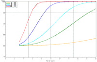 c
c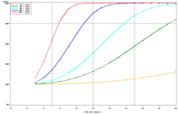 d
d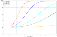
 b
b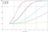
 b
b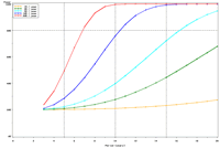 c
c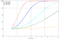 d
d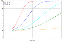 a
a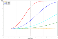 b
b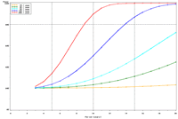 c
c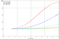 d
d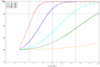 e
e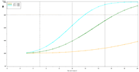 a
a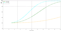 b
b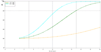 c
c