Conservation Ecology - Population Demographic Models for the Conservation of Endangered Indiana Bats

Model Details

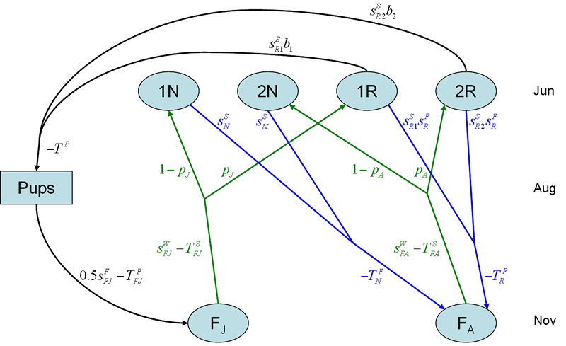
Stage 1. The modeling process will occur in 4 steps, or stages. Stage 1 will accommodate the dynamics of a single recovery unit with the population of bats ostensibly using a single hibernacula for overwintering (Figure 1).

In Stage 1 (Figure 1), there are four age-reproductive classes, non-reproductive yearlings (1N), non-reproductive adults (2N), reproductive yearlings (1R), and reproductive adults (2R).Males are ignored in this first stage of model development. Each reproductive class (1R and 2R) will produce some proportion of pups, as determined by a class-specific recruitment rate and a class-specific summer survival rate. Some total number of pups are potentially removed (through a take). These pups in turn experience a fall survival and potentially another absolute take. Upon survival through the fall, the juveniles are partitioned into non-reproductive yearlings and reproductive yearlings after experiencing an overwinter survival probability and a potential spring take.Adults similarly incur an overwinter survival probability and a spring take, before being partitioned into non-reproductive and reproductive classes.After completion of the first year, yearlings incur a summer survival and potential take before reaching adulthood.

An important point to make here is that survival rates are relative to N, the size of the population within the recovery unit. Take, however, is absolute; thus, while survival may be on the order of, say, 75%, take will involve the removal of x number of individuals, 50 for instance.

Expert opinion will be used to provide initial point parameter estimates for survival (s), reproductive success (b), take (T), and the propensity to reproduce (p). Experts consulted will initially comprise those attending the structured decision-making workshop that motivates this research effort. At the first stage, elicitation of expert opinion will be informal. Given initial values for the parameter estimates, the form and function of this model will be examined by determining where major sensitivities in the model occur; further, we should be able to conduct initial assessments of the risk of extinction for this species.

Results of this stage will describe the probability of quasi-extinction, i.e., the time at which the species is expected to become extinct given the particular dynamics of the population. We describe this phenomenon as quasi-extinction rather than extinction because we do not consider (non-linear) small population dynamics (e.g., Allee effects) which may hasten or ameliorate processes occurring in the larger population dynamics that we are concerned with in this present study. Quasi-extinction will be calculated for a single recovery unit at this initial stage. For scenario assessment, the change in the probability of quasi-extinction between scenarios will be calculated.

To accommodate assessments relating to recovery, we will report 10-yr projected growth rates given the parameter estimates of the scenario. We will also report the recovery-unit minimum population in winter.

Stage 2. In stage 1, we assume point estimates for parameters. Potentially the most difficult stage for programming will be stage 2, where uncertainty in parameter estimates will be allowed. We will allow users to specify expected ranges of variation in survival (s), reproductive success (b), take (T), and the propensity to reproduce (p). At the conclusion of this stage, model results will include measures of uncertainty resulting from parameter uncertainty.

For scenario assessment, this range of variation or uncertainty can play out in one of two ways. In one case, the user will provide a range of variation for each of the model parameters and a point-level estimate for the effect of some action on the population. For instance, a user may wish to evaluate the impact of white-nose syndrome on a population. In this case, a baseline will be prepared with expected ranges of variation in s, b, T, and p. The white-nose syndrome scenario may be examined by modifying overwinter survival to some much lower point estimate (reducing s from some baseline of 0.8 to some putative level of 0.05, but maintaining the magnitude of variation in the uncertainty associated with the baseline). In another case, the user may be uncertain as to the effect of white-nose syndrome, so they may wish to allow for uncertainty in the scenario value which may be greater than the uncertainty occurring in the baseline. Thus, the range of variation may be amended to reflect this greater uncertainty (A further alternative is to hold the baseline parameters constant and to allow uncertainty in the scenario effect, to ascertain the effect of the user’s uncertainty on population performance).

A last element to Stage 2 will include incorporation of pre-programmed effects of environmental and catastrophic stochasticity, with particular reference to the effects of white-nose syndrome on the Indiana bat population. Environmental stochasticity will be allowed to play out in its effect on survival (s) and reproductive (b) rates; catastrophic stochasticity will occur in the hibernacula-specific winter survival (s) rates. Full elaboration of environmental and catastrophic uncertainty will occur through the end of Stage 4.

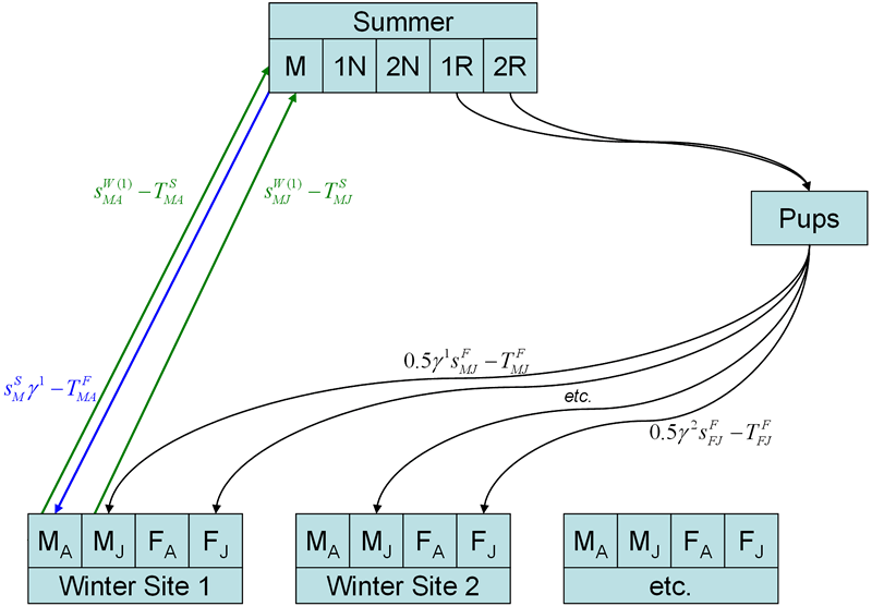
Stage 3. This stage primarily elaborates the number of hibernacula to which the bats are partitioned. In Stage 1, we assumed a single hibernaculum. In Stage 3, we will initially model two hibernacula. We intend to allow for a user-specified number of hibernacula to partition the population. We intend to allow users to specify the number of hibernacula because this number varies by recovery unit and hypotheses exist suggesting multiple hibernacula are important for population survival. An additional layer of complexity will be the inclusion of males, both as adults and juveniles.

Unlike Stage1, probability of quasi-extinction will be calculable for both the individual recovery unit and for the ensemble of recovery units (i.e., a probability of range-wide extinction).

Stage 4. The final stage of model development will primarily be associated with making the software more user friendly.By this stage, the user group will have been provided earlier prototypes and in turn given their feedback. As best as is possible, this feedback will be used to amend the user interface. For instance, the user group will identify a number of scenarios (including their parameter estimates and expected ranges of variation) to include pre-programmed into the software. Further, at this stage of development, the principal investigator with the assistance of the programmer will provide a user’s guide to the software.

Figure 1. (Reproduced from Szymanski et al., unpublished document) Schematic life-cycle diagram for the Indiana bat population model, female segment only and without spatial structure. The winter state variables (number of juvenile females, FJ; and number of adult females, FA) are measured in November, just at the beginning of hibernation. The summer state variables (number of non-reproductive yearlings, 1N; number of non-reproductive older adults, 2N; number of reproductive yearlings, 1R; and number of reproductive older adults, 2R) are measured in June, just before parturition. Pups is an intermediate state variable, measured at volancy. The transitions from winter to summer are shown in green, and include overwinter survival (sW), spring take (TS), and propensity to reproduce. The transitions from summer to winter are shown in blue, and include summer survival (sS), fall survival (sF), and fall take (TF). The reproductive transitions are shown in black, and include summer survival of reproductive females (sS), reproductive rates (b), take of pups (TP), fall juvenile survival ( formula 1

), and fall take of juveniles ( formula 2

). Note that lowercase transition rates (s, b, and p) are multipliers to the size of the population segment being affected; while uppercase transition parameters (T) are absolute measures of take.

Figure 2. (Reproduced from Szymanski et al., unpublished document) Schematic life-cycle diagram (incomplete) for the Indiana bat population model, including spatial structure and all sex- and age-classes. Note that the female transitions are not shown (see Fig. 1) and not all of the spatial transitions are drawn. The desired model will be structured at the regional level, with a single regional summer population, but several distinct winter populations (e.g., primary hibernacula tracked separately, and the remainder of the winter population combined into a final “site”). Winter survival rates may depend on the site. The spatial structure requires an additional set of parameters (the g’s) to govern the distribution of the summer population to the winter sites. In the model, take of absolute numbers of animals can occur at three points: “spring” take (TS) includes late winter take, take during spring migration, and pre-reproductive (pre-volancy) take on the breeding grounds; “fall” take (TF) includes take during fall migration, swarming, and early winter; and pup take (TP) includes take of pre-volant pups without concurrent take of the mother.

Szymanski, J. A., L. Pruitt, M. C. Runge, M. Armstrong, R. A. King, C. Mcgowan, R. Niver, D. Sparks, and D. C. Brewer. 2009. Developing performance criteria for a population model for Indiana Bat conservation. A case study from the structured decision making workshop, December 8–12, 2008, National Conservation Training Center, Shepherdstown, West Virginia, USA.