Decision Support Systems
Curve Fit: A Pixel Level Raster Regression Tool
Download Curve Fit 10.1
Sample Data
Curve Fit Installation and Use Instructions (.pdf)
Curve Fit is an extension to the GIS application ArcMap that allows the user to run regression analysis on a series of raster datasets (geo-referenced images). The user enters an array of values for an explanatory variable (X). A raster dataset representing the corresponding response variable (Y) is paired with each X value entered by the user. Curve Fit then uses either linear or nonlinear regression techniques (depending on user selection) to calculate a unique mathematical model at each pixel of the input raster datasets. Curve Fit outputs raster surfaces of parameter estimate, error, and multi-model inference. Curve Fit is both an explanatory and predictive tool that provides spatial modelers with the ability to perform key statistical functions at the finest scale. Some examples of hypothetical Curve Fit applications are: habitat variety as a function of scale, population density as a function of time, or current velocity as a function of discharge rate (see detailed example below).
Curve Fit Performs Both Linear and Nonlinear Regression Analysis:
Curve Fit uses both linear and nonlinear regression techniques. If a nonlinear model is selected the user will have the option to constrain parameters and manipulate solution iterations and tolerances.
Linear Regression Models:
|
 Linear: Linear:  simple, powerful, and easy to interpret simple, powerful, and easy to interpret
|
 Polynomial: Polynomial:  degree specified by the user, resultant curves are morphologically diverse degree specified by the user, resultant curves are morphologically diverse
|
Nonlinear Regression Models:
|
 Power: Power:  often used to model growth and decay often used to model growth and decay
|
 Exponential: Exponential:  often used to model growth and decay often used to model growth and decay
|
 Four Parameter Logistic: Four Parameter Logistic: 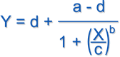 produces a sigmoidal curve defined by lower and upper asymptotes (a, d), a midpoint (c), and the slope (b) measured at the midpoint produces a sigmoidal curve defined by lower and upper asymptotes (a, d), a midpoint (c), and the slope (b) measured at the midpoint
|
Curve Fit Produces Raster Products Describing Goodness of Fit, Multi-Model Inference, Parameter Estimate, and Error Estimate:
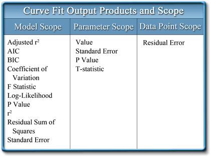
Curve Fit output products cover three scopes: model, parameter, and data point (Table 1). The model scope contains statistical products that evaluate model fit, error, null hypothesis testing, and products used to select and compare between multiple models. The parameter scope contains: parameter value estimate, standard error, P-value, and T-statistic. The data point scope contains only one class of output product, residual error.
Each output product is a raster dataset matching the resolution and extent of the input datasets. The user can select output formats of 64 bit double precision or 32 bit single precision. A single run of Curve Fit can produce an enormous volume of data. Therefore it pays to be judicious when selecting analysis products. |
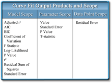
Table 1. Curve Fit Output Products and Scope |
| |
|
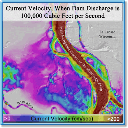
Example Analysis: Current Velocity as a Function of Dam Discharge for Pool 8 of the Upper Mississippi River |
Ten raster layers were used as input in this example, each representing a current velocity at a specific discharge rate for Pool 8 of the Upper Mississippi River (Figure 2). Rates ranged from 10,000 cubic feet per second (cfs) to 100,000 cfs, and were calculated at 10,000 cfs intervals using a Surface-water Modeling System (SMS). These data were then loaded into Curve Fit and modeled using a 3rd degree polynomial. |
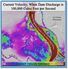
Figure 2. 1 of 10 current velocity input layers used in the regression analysis |
| |
|
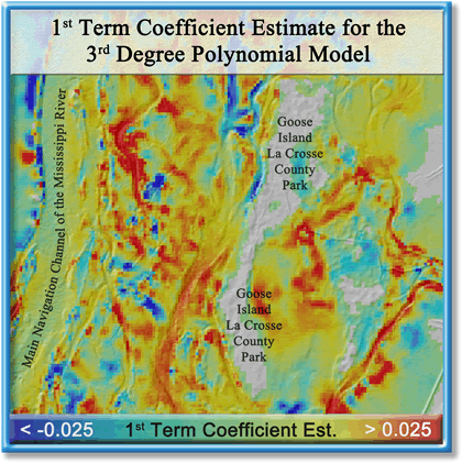
| The Curve Fit output products selected for this example included: coefficient estimates for the 1st, 2nd, 3rd, and 4th terms of the polynomial and the adjusted r2 product. The coefficient estimates (Figure 3) can be used as a surrogate to the SMS modeling process. With these estimates in hand, the user can use a GIS to calculate current velocity at any intermediate discharge rate. This greatly simplifies the modeling process and opens up current velocity modeling to those who do not possess or who are not proficient with a surface-water modeling system. |

Figure 3. 1 of 4 coefficient estimates comprising the fitted polynomial model |
| |
|
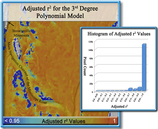
| The adjusted r2 output and accompanying histogram (Figure 4) show that the majority of the polynomials modeled within the analysis area explain >90% of the variation within the input data. Although these are exceptional results, one could choose to rerun Curve Fit using a different curve or a polynomial of a different degree and compare model fit between the results. |
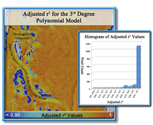
Figure 4. Adjusted r2 output layer and histogram |
Point of contact: Tim Fox
Funded by the USGS and the U.S. Army Corps of Engineers’ Upper Mississippi River Restoration—Environmental Management Program
|